GSEA
Connor H Knight
11/08/2021
GSEA.RmdPerfoming gene set enricvhment with ssGSEA
Gene Set Enrichment Analysis enables us to determine if a defined set of genes shows a statistically difference between biological states. Here we apply this on single-cell RNA-seq data. In this tutorial, we show you how to enrich certain pathways in your single-cell data.
Running GSEA
We begin by loading some test data: This command is simple loading in some example data and inserting it into an IBRAP object.
library(IBRAP)
#> Welcome to IBRAP

system('curl -LJO https://raw.githubusercontent.com/connorhknight/IBRAP/main/data/celseq2.rds')

celseq2 <- readRDS('celseq2.rds')

obj <- createIBRAPobject(counts = celseq2$counts, original.project = 'celseq2', meta.data = celseq2$metadata)

obj <- perform.sct(object = obj)
obj <- perform.pca(object = obj, assay = 'SCT')
obj <- perform.umap(object = obj, assay = 'SCT', reduction = 'PCA', dims.use = list(20))
We next next need to gather gene sets:
There are a couple of ways to do this: (1) get the gene sets from the escape package or (2) define your own.
# Option 1

gene.sets <- escape::getGeneSets(library = 'H', species = 'Homo sapiens')

# Option 2

gene.sets <- list(Tcell_signature = c("CD2","CD3E","CD3D"),
                  Myeloid_signature = c("SPI1","FCER1G","CSF1R"))
gene.sets <- escape::getGeneSets(library = 'H', species = 'Homo sapiens')

# You can adjust the number of computing cores to dedicate to the calculations throguh the core parameter.

results <- perform.gsea(object = obj, gene.sets = gene.sets, return_object = F)
#> [1] "Using sets of 1000 cells. Running 3 times."
#> Setting parallel calculations through a SnowParam back-end
#> with workers=6 and tasks=100.
#> Estimating ssGSEA scores for 50 gene sets.
#> Setting parallel calculations through a SnowParam back-end
#> with workers=6 and tasks=100.
#> Estimating ssGSEA scores for 50 gene sets.
#> Setting parallel calculations through a SnowParam back-end
#> with workers=6 and tasks=100.
#> Estimating ssGSEA scores for 50 gene sets.

# We can then bind the results into our IBRAP object metadata.

obj@sample_metadata <- cbind(obj@sample_metadata, results)Heatmaps
Firstly, we convert our IBRAP object into a SCE object to be compatible with dittoseq.
library(dittoSeq)
#> Loading required package: ggplot2

dittoseq_obj <- prepare.for.dittoSeq(object = obj, assay = 'SCT', slot = 'normalised', reduction = 'PCA_UMAP', clust.method = 'metadata')
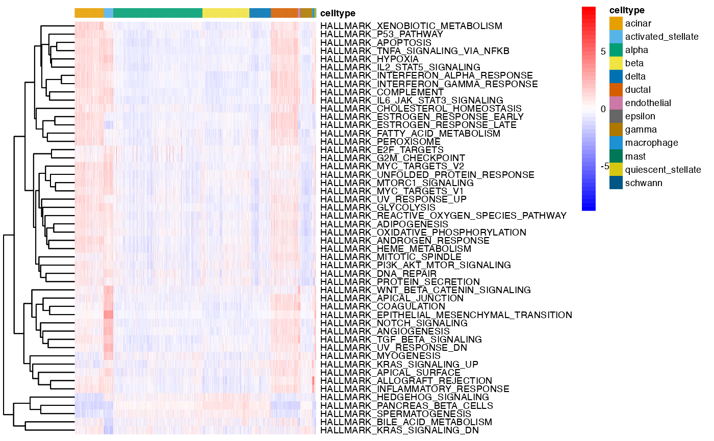
Then, we plot our metaprogrammes in a heatmap.
dittoHeatmap(dittoseq_obj, genes = NULL, metas = names(results),
             annot.by = "celltype",
             fontsize = 7)
There are many other plots that can be performed on enrichment analysis which can be found in the following tutorial: http://www.bioconductor.org/packages/release/bioc/vignettes/escape/inst/doc/vignette.html