Automated Annotation
Connor H Knight & Faraz Khan
11/08/2021
singleR_annotation.RmdIn our previous tutrols we have taught you how to cluster cells by similarity and then interpret their cell types through gene expression interpretation. However, a different methodology to label cell types is avaialble. This method is called supervised clustering, where a reference dataset is obtained and used to identify the cell types in a query dataset.
Automated cell type annotation
Well-analysed reference maps are currently emerging in single-cell data. To take advantage of this, reference-based cell type annotation algorithms are being developed. Thus, we included SingleR into IBRAP which enables the user to bypass downstream analyses and annotate new datasets more rapidly.
A pre-requisite for automated annotation is intuitive - the reference sample must have correct cell type labels.
For this analysis we will use pancreatic cell samples analysed using smartseq2 and celseq2, these can be acquired from the following links:
https://www.dropbox.com/s/heughk2kl0lg6qc/smartseq2.rds?dl=0 https://www.dropbox.com/s/txlq7875wkthb3y/celseq2.rds?dl=0
We can annotate either dataset using the other. In this tutorial, we will use the smartseq2 sample as a reference to annotate the cekseq2 sample.
The query and reference matrix is either log (end bias) or tpm & log (full-length) transformed to normalise the data. reference cell type labels must then be provided using the ref.label paramter in the same order as the columns of the reference matrix. SingleR will sequence through each singular query cell and iterate a probability analysis to identify the most probable cell type.
celseq2_items <- readRDS(file.choose())
smartseq2_items <- readRDS(file.choose())

celseq2 <- createIBRAPobject(counts = celseq2_items$counts,
                             meta.data = celseq2_items$metadata,
                             original.project = 'celseq2',
                             method.name = 'RAW',
                             min.cells = 3,
                             min.features = 200)

celseq2 <- perform.singleR.annotation(object = celseq2_items,
                                      assay = 'RAW',
                                      slot = 'counts',
                                      ref = as.matrix(smartseq2_items$counts),
                                      log.transform = T,
                                      ref.labels = smartseq2_items$metadata$celltype)
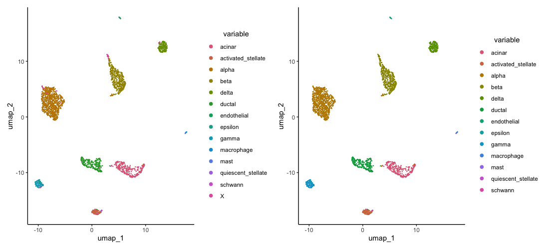
SingleR annotation results will be added the object@sample_metadata. Two columns are produced one with labels and another with pruned labels. The difference is that the pruned labels will add an X for cells that it is not highly certain of whereas, the labels one will label every cell with its closest cell type - even if it is not highly certain. We can now observe the results:
celseq2 <- perform.sct(object = celseq2,
                    assay = 'RAW',
                    slot = 'counts')

celseq2 <- perform.pca(object = celseq2,
                    assay = 'SCT',
                    n.pcs = 50, reduction.save = 'pca')

celseq2 <- perform.umap(object = celseq2,
                     assay = 'SCT',
                     reduction = 'pca',
                     n_components = 3,
                     n.dims = list(1:10))

plot1 <- plot.reduced.dim(object = celseq2, reduction = 'pca_umap', assay = 'SCT', clust.method = 'metadata', column = 'singleR_pruned_labels_1', pt.size = 0.1)

plot2 <- plot.reduced.dim(object = celseq2, reduction = 'pca_umap', assay = 'SCT', clust.method = 'metadata', column = 'singleR_labels_1', pt.size = 0.1)

plot1 + plot2
Here, we have used our smartseq2 dataset labels to label our celseq2 dataset in a much easier and faster way. However, this method has limitations since it can only label cell types that are present in the reference dataset.